Back propagation
Contents
Back propagation
In this chapter we show in detail how to carry out supervised learning for multilayer classifiers discussed in chapter More layers. Since the method is based on minimizing the number of erroneous answers on a test sample, we begin with a thorough discussion of the problem of error minimization in our setup.
Minimizing the error
Recall that in our example with points on the plane from chapter Perceptron, the condition for the pink points was given by the inequality
\(w_0+w_1 x_1 + w_2 x_2 > 0\).
We have already briefly mentioned the equivalence class related to dividing this inequality with a positive constant \(c\). In general, at least one of the weights in the condition must be nonzero to have a nontrivial condition. Suppose or definiteness that \(w_0 \neq 0\) (other cases may be treated analogously). Then we can divide both sides of the inequality with \(|w_0|\) to obtain
Introducing the short-hand notation \(v_1=\frac{w_1}{w_0}\) and \(v_2=\frac{w_2}{w_0}\), this can be rewritten in the form
where the sign \({\rm sgn}(w_0) = \frac{w_0}{|w_0|}\), hence we effectively have a two-parameter system (for each sign of \(w_0\)).
Obviously, with some values of \( v_1 \) and \( v_2 \) and for a given point from the data sample, the perceptron provides a correct or incorrect answer. It is thus natural to define the error function \(E\) such that each point of \(p\) from the sample contributes 1 if the answer is incorrect, and 0 if it is correct:
\(E\) is thus interpreted as the number of misclassified points.
We can easily construct this function in Python:
def error(w0, w1 ,w2, sample, f=func.step):
    """
    error function for the perceptron (for 2-dim data with labels)

    inputs:
    w0, w1, w2 - weights
    sample - array of labeled data points p
             p in an array in the format [x1, x1, label]
    f - activation function

    returns:
    error
    """
    er=0                                       # initial value of the error
    for i in range(len(sample)):               # loop over data points
        yo=f(w0+w1*sample[i,0]+w2*sample[i,1]) # obtained answer
        er+=(yo-sample[i,2])**2
                      # sample[i,2] is the label
                      # adds the square of the difference of yo and the label
                      # this adds 1 if the answer is incorrect, and 0 if correct
    return er  # the error
Actually, we have used a little trick here, in view of the future developments. Denoting the obtained result for a given data point as \(y_o^{(p)}\) and the true result (label) as \(y_t^{(p)}\) (both have values 0 or 1), we may write equivalently
which is the formula programmed above. Indeed, when \(y_o^{(p)}=y_t^{(p)}\) (correct answer) the contribution of the point is 0, and when \(y_o^{(p)}\neq y_t^{(p)}\) (wrong answer) the contribution is \((\pm 1)^2=1\).
We repeat the simulations of chapter Perceptron to generate the labeled data sample samp2 of 200 points (the sample is built with \(w_0=-0.25\), \(w_1=-0.52\), and \(w_2=1\), which corresponds to \(v_1=2.08\) and \(v_2=-4\), with \({\rm sgn}(w_0)=-1\)).
We now need again the perceptron algorithm of section Perceptron algorithm. In our special case, it operates on a sample of two-dimensional labeled data. For convenience, a single round of the algorithm can be collected into a function as follows:
def teach_perceptron(sample, eps, w_in, f=func.step):
    """
    Supervised learning for a single perceptron (single MCP neuron)
    for a sample of 2-dim. labeled data

    input:
    sample - array of two-dimensional labeled data points p
             p is an array in the format [x1,x2,label]
             label = 0 or 1
    eps    - learning speed
    w_in   - initial weights in the format [[w0], [w1], [w2]]
    f      - activation function

    return: updated weights in the format [[w0], [w1], [w2]]
    """
    [[w0],[w1],[w2]]=w_in         # define w0, w1, and w2
    for i in range(len(sample)):  # loop over the whole sample
        for k in range(10):       # repeat 10 times

            yo=f(w0+w1*sample[i,0]+w2*sample[i,1]) # output from the neuron, f(x.w)

            # update of weights according to the perceptron algorithm formula
            w0=w0+eps*(sample[i,2]-yo)*1
            w1=w1+eps*(sample[i,2]-yo)*sample[i,0]
            w2=w2+eps*(sample[i,2]-yo)*sample[i,1]

    return [[w0],[w1],[w2]]       # updated weights
Next, we trace the action of the perceptron algorithm, watching how it modifies the error function \(E(v_1,v_2)\) introduced above. We start from random weights, and then carry out 10 rounds of the above-defined teach_perceptron function, printing out the updated weights and the corresponding error:
weights=[[func.rn()], [func.rn()], [func.rn()]] # initial random weights

print("Optimum:")
print("   w0  w1/w0  w2/w0 error")   # header

eps=0.7                 # initial learning speed
for r in range(10):     # rounds
    eps=0.8*eps         # decrease the learning speed
    weights=teach_perceptron(samp2,eps,weights,func.step)
                        # see the top of this chapter

    w0_o=weights[0][0]  # updated weights and ratios
    v1_o=weights[1][0]/weights[0][0]
    v2_o=weights[2][0]/weights[0][0]

    print(np.round(w0_o,3),np.round(v1_o,3),np.round(v2_o,3),
          np.round(error(w0_o, w0_o*v1_o, w0_o*v2_o, samp2, func.step),0))
Optimum:
   w0  w1/w0  w2/w0 error
-0.297 3.643 -7.231 22.0
-0.745 2.493 -3.373 28.0
-0.745 2.201 -4.032 0.0
-0.745 2.201 -4.032 0.0
-0.745 2.201 -4.032 0.0
-0.745 2.201 -4.032 0.0
-0.745 2.201 -4.032 0.0
-0.745 2.201 -4.032 0.0
-0.745 2.201 -4.032 0.0
-0.745 2.201 -4.032 0.0
We note that in subsequent rounds the error gradually decreases (depending on a simulation, it can sometimes jump up if the learning speed is too large, but this is not a problem as long as we can get down to the minimum), reaching a final value which is very small or 0 (depending on the particular instance of simulation). Therefore the perceptron algorithm, as we already experienced in chapter Perceptron, minimizes the error on the training sample.
It is illuminating to look at a contour map of the error function \(E(v_1, v_2)\) in the vicinity of the optimal parameters:
fig, ax = plt.subplots(figsize=(3.7,3.7),dpi=120)

delta = 0.02  # grid step in v1 and v2 for the contour map
ran=0.8       # plot range around (v1_o, v2_o)

v1 = np.arange(v1_o-ran,v1_o+ran, delta) # grid for v1
v2 = np.arange(v2_o-ran,v2_o+ran, delta) # grid for v2
X, Y = np.meshgrid(v1, v2)               # mesh for the contour plot

Z=np.array([[error(-1,-v1[i],-v2[j],samp2,func.step)
             # we use the scaling property of the error function here
             for i in range(len(v1))] for j in range(len(v2))]) # values of E(v1,v2)

CS = ax.contour(X, Y, Z, [1,5,10,15,20,25,30,35,40,45,50])
                        # explicit contour level values

ax.clabel(CS, inline=1, fmt='%1.0f', fontsize=9) # contour label format

ax.set_title('Error function', fontsize=11)
ax.set_aspect(aspect=1)

ax.set_xlabel('$v_1$', fontsize=11)
ax.set_ylabel('$v_2$', fontsize=11)

ax.scatter(v1_o, v2_o, s=20,c='red',label='found minimum') # our found optimal point

ax.legend()
plt.show()
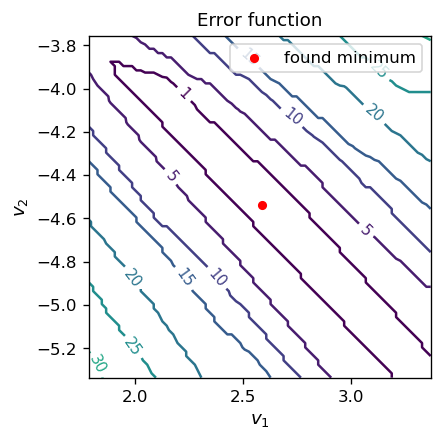
The obtained minimum is inside (or close to, depending on the simulation) an elongated region of \( v_1 \) and \( v_2\) where the error vanishes.
Continuous activation function
Looking closely at the contour map above, we can see that the lines are “serrated”. This is because the error function, for an obvious reason, assumes integer values. It is therefore discontinuous and hence non-differentiable. The discontinuities originate from the discontinuous activation function, i.e. the step function. Having in mind the techniques we will get to know soon, it is advantageous to use continuous activation functions. Historically, the so-called sigmoid
has been used in many practical applications of ANNs.
# sigmoid, a.k.a. the logistic function, or simply (1+arctanh(-s/2))/2
def sig(s):
    return 1/(1+np.exp(-s))
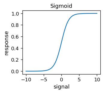
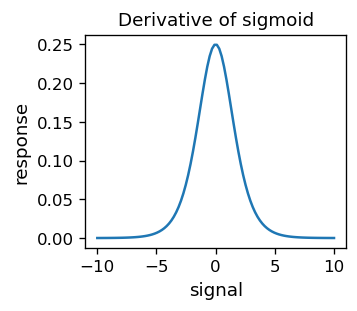
This function is of course differentiable. Moreover,
which is its special feature.
# derivative of sigmoid
def dsig(s):
     return sig(s)*(1-sig(s))
A sigmoid with “temperature” \( T \) is also introduced (this nomenclature is associated with similar expressions for thermodynamic functions in physics):
# sigmoid with temperature T
def sig_T(s,T):
    return 1/(1+np.exp(-s/T))
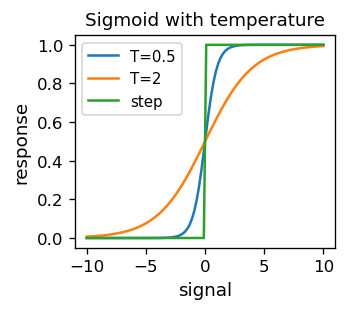
For smaller and smaller \(T\), the sigmoid approaches the previously used step function.
Note that the argument of the sigmoid is the quotient
which means that we can always take \( T = 1 \) without losing generality (\( T \) is the “scale”). However, we now have three independent arguments \( \xi_0 \), \( \xi_1 \), and \( \xi_2\), so it is impossible to reduce the present situation to only two independent parameters, as was the case in the previous section.
We now repeat our example with the classifier, but with the activation function given by the sigmoid. The error function, with the answers
becomes
We run the perceptron algorithm with the sigmoid activation function 1000 times, printing out every 100th step:
weights=[[func.rn()],[func.rn()],[func.rn()]]      # random weights from [-0.5,0.5]

print("   w0   w1/w0  w2/w0 error")   # header

eps=0.7                       # initial learning speed
for r in range(1000):         # rounds
    eps=0.9995*eps            # decrease learning speed
    weights=teach_perceptron(samp2,eps,weights,func.sig) # update weights
    if r%100==99:
        w0_o=weights[0][0]               # updated weights
        w1_o=weights[1][0]
        w2_o=weights[2][0]
        v1_o=w1_o/w0_o                   # ratios of weights
        v2_o=w2_o/w0_o
        print(np.round(w0_o,3),np.round(v1_o,3),np.round(v2_o,3),
              np.round(error(w0_o, w0_o*v1_o, w0_o*v2_o, samp2, func.sig),5))
   w0   w1/w0  w2/w0 error
-16.036 2.665 -4.64 0.37383
-19.825 2.627 -4.588 0.25397
-22.375 2.595 -4.547 0.19764
-24.308 2.572 -4.52 0.16604
-25.869 2.555 -4.501 0.14589
-27.178 2.541 -4.487 0.13176
-28.306 2.531 -4.476 0.12106
-29.293 2.523 -4.467 0.11244
-30.169 2.516 -4.46 0.10517
-30.952 2.511 -4.454 0.09883
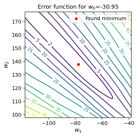
We notice, as expected, a gradual decrease of the error as the simulation proceeds. Since the error function now has three independent arguments, it cannot be drawn in two dimensions. We can, however, show its projection, e.g. with a fixed value of \( w_0 \), which we do below:
fig, ax = plt.subplots(figsize=(3.7,3.7),dpi=120)

delta = 0.5
ran=40
r1 = np.arange(w1_o-ran, w1_o+ran, delta)
r2 = np.arange(w2_o-ran, w2_o+ran, delta)
X, Y = np.meshgrid(r1, r2)

Z=np.array([[error(w0_o,r1[i],r2[j],samp2,func.sig)
             for i in range(len(r1))] for j in range(len(r2))])

CS = ax.contour(X, Y, Z,[0,2,5,10,15,20,25,30,35,40,45,50])
ax.clabel(CS, inline=1, fmt='%1.0f', fontsize=9)

ax.set_title('Error function for $w_0$='+str(np.round(w0_o,2)), fontsize=11)
ax.set_aspect(aspect=1)
ax.set_xlabel('$w_1$', fontsize=11)
ax.set_ylabel('$w_2$', fontsize=11)

ax.scatter(w1_o, w2_o, s=20,c='red',label='found minimum') # our found optimal point

ax.legend()
plt.show()
Note
As we carry out more and more iterations, we notice that the magnitude of weights becomes lager and lager, while the error naturally gets smaller. The reason is following: our data sample is separable, so in the case when the step function is used for activation, it is possible to separate the sample with the dividing line and get down with the error all the way to zero. In the case of the sigmoid, there is always some (tiny) contribution to the error, as the values of the function are in the range (0,1). As we have discussed above, in the sigmoid, whose argument is \( (w_0 + w_1 x_1 + w_2 x_2) / T\), increasing the weights is equivalent to scaling down the temperature \(T\). Then, ultimately, the sigmoid approaches the step function, and the error tends to zero. Precisely this behavior is seen in the simulations above.
Steepest descent
The reason of carrying out the above simulations was to drive the reader into conclusion that the issue of optimizing the weights can be reduced to a generic problem of minimizing a multi-variable function. This is a standard (though in general difficult) problem in mathematical analysis and numerical methods. Issues associated with finding the minimum of multivariable functions are well known:
there may be local minima, and therefore it may be very difficult to find the global minimum;
the minimum can be at infinity (that is, it does not exist mathematically);
The function around the minimum can be very flat, such that the gradient is very small, and the update in gradient methods is extremely slow;
Overall, numerical minimization of functions is an art! Many methods have been developed and a proper choice for a given problem is crucial for success. Here we apply the simplest variant of the steepest descent method.
For a differentiable function of multiple variables, \( F (z_1, z_2, ..., z_n) \), locally the steepest slope is defined by minus the gradient of the function \( F \),
where the partial derivatives are defined as the limit
and similarly for the other \( z_i \).
The method of finding the minimum of a function by the steepest descent is given by an iterative algorithm, where we update the coordinates (of a searched minimum) at each iteration step \(m\) (shown in superscripts) with
We need to minimize the error function
The chain rule is used to evaluate the derivatives.
Chain rule
For a composite function
\([f(g(x))]' = f'(g(x)) g'(x)\).
For a composition of more functions \([f(g(h(x)))]' = f'(g(h(x))) \,g'(h(x)) \,h'(x)\), etc.
This yields
(derivative of square function \( \times \) derivative of the sigmoid \( \times \) derivative of \( s ^ {(p)} \)), where we have used the special property of the sigmoid derivative in the last equality. The steepest descent method updates the weights as follows:
Note that updating always occurs, because the response \( y_o^ {(p)} \) is never strictly 0 or 1 for the sigmoid, whereas the true value (label) \( y_t ^ {(p)} \) is 0 or 1.
Because \( y_o ^ {(p)} (1-y_o ^ {(p)}) = \sigma (s ^ {(p)}) [1- \sigma (s ^ {(p)})] \) is far from zero only around \( s ^ {(p)} = \) 0 (see the sigmoid’s derivative plot earlier), a significant updating occurs only near the threshold. This is fine, as the “problems” with misclassification happen near the dividing line.
Note
In comparison, the earlier perceptron algorithm is structurally very similar,
but here the updating occurs with all the points from the sample, not just near the threshold.
The code for the learning algorithm of our perceptron with the steepest descent update of weights is following:
def teach_sd(sample, eps, w_in): # Steepest descent for the perceptron

    [[w0],[w1],[w2]]=w_in              # initial weights
    for i in range(len(sample)):       # loop over the data sample
        for k in range(10):            # repeat 10 times

            yo=func.sig(w0+w1*sample[i,0]+w2*sample[i,1])  # obtained answer for pont i

            w0=w0+eps*(sample[i,2]-yo)*yo*(1-yo)*1            # update of weights
            w1=w1+eps*(sample[i,2]-yo)*yo*(1-yo)*sample[i,0]
            w2=w2+eps*(sample[i,2]-yo)*yo*(1-yo)*sample[i,1]
    return [[w0],[w1],[w2]]
Its performance is similar to the original perceptron algorithm studied above:
weights=[[func.rn()],[func.rn()],[func.rn()]]      # random weights from [-0.5,0.5]

print("   w0   w1/w0  w2/w0 error")   # header

eps=0.7                       # initial learning speed
for r in range(1000):         # rounds
    eps=0.9995*eps            # decrease learning speed
    weights=teach_sd(samp2,eps,weights) # update weights
    if r%100==99:
        w0_o=weights[0][0]               # updated weights
        w1_o=weights[1][0]
        w2_o=weights[2][0]
        v1_o=w1_o/w0_o
        v2_o=w2_o/w0_o
        print(np.round(w0_o,3),np.round(v1_o,3),np.round(v2_o,3),
              np.round(error(w0_o, w0_o*v1_o, w0_o*v2_o, samp2, func.sig),5))
   w0   w1/w0  w2/w0 error
-8.15 2.655 -4.624 1.15014
-10.036 2.651 -4.617 0.81162
-11.286 2.64 -4.601 0.66387
-12.231 2.629 -4.587 0.57811
-12.992 2.62 -4.575 0.52091
-13.63 2.612 -4.565 0.47946
-14.178 2.605 -4.556 0.44769
-14.658 2.598 -4.549 0.42237
-15.084 2.593 -4.542 0.40159
-15.466 2.588 -4.536 0.38416
To summarize the development up to now, we have shown that one can teach a single-layer perceptron (single MCP neuron) efficiently with the help of the steepest descent method, minimizing the error function generated with the test sample. In the next section we generalize this idea to any multi-layer feed-forward ANN.
Backprop algorithm
The material of this section is absolutely crucial for understanding of the idea of training neural networks via supervised learning. At the same time, it can be quite difficult for a reader less familiar with mathematical analysis, as there appear derivations and formulas with rich notation. However, we could not find a way to present the material in a simpler way than below, keeping the necessary rigor.
Note
The formulas we derive step by step here constitute the famous back propagation algorithm (backprop) [BH69] for updating the weights of a multi-layer perceptron. It uses just two ingredients:
the chain rule for computing the derivative of a composite function, already used above, and
the steepest descent method, explained in the previous lecture.
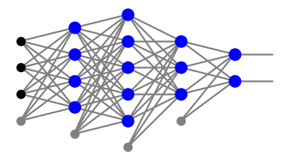
Consider a perceptron with any number of neuron layers, \(l\). The neurons in intermediate layers \(j=1,\dots,l-1\) are numbered with corresponding indices \(\alpha_j=0,\dots,n_j\), with 0 indicating the bias node. In the output layer, having no bias node, the numbering is \(\alpha_l=1,\dots,n_l\). For example, the network form the plot below has
with the indices in each layer counted from the bottom.
The error function is a sum over the points of the training sample and, additionally, over the nodes in the output layer:
where \( \{w \} \) represent all the network weights. A single point contribution to \(E\), denoted as \( e \), is a sum over all the neurons in the output layer:
where we have dropped the superscript \((p)\) for brevity. For neuron \(\alpha_j\) in layer \(j\) the entering signal is
The outputs from the output layer are
whereas the output signals in the intermediate layers \(j=1,\dots,l-1\) are
with the bias node having the value 1.
Subsequent explicit substitutions of the above formulas into \(e\) are as follows:
\(e = \sum_{{\alpha_l}=1}^{n_l}\left( y_{o,{\alpha_l}}-y_{t,{\alpha_l}}\right)^2\)
\(=\sum_{{\alpha_l}=1}^{n_l} \left( f \left (\sum_{\alpha_{l-1}=0}^{n_{l-1}} x_{\alpha_{l-1}}^{l-1} w_{\alpha_{l-1} {\alpha_l}}^{l} \right )-y_{t,{\alpha_l}} \right)^2\)
\(=\sum_{{\alpha_l}=1}^{n_l} \left( f \left (\sum_{\alpha_{l-1}=1}^{n_{l-1}} f \left( \sum_{\alpha_{l-2}=0}^{n_{l-2}} x_{\alpha_{l-2}}^{l-2} w_{\alpha_{l-2} \alpha_{l-1}}^{l-1}\right) w_{\alpha_{l-1} {\alpha_l}}^{l} + x_0^{l-1} w_{0 \gamma}^{l} \right)-y_{t,{\alpha_l}} \right)^2\)
\(=\sum_{{\alpha_l}=1}^{n_l} \left( f \left (\sum_{\alpha_{l-1}=1}^{n_{l-1}} f\left( \sum_{\alpha_{l-2}=1}^{n_{l-2}} f\left( \sum_{\alpha_{l-3}=0}^{n_{l-3}} x_{\alpha_{l-3}}^{l-3} w_{\alpha_{l-3} \alpha_{l-2}}^{l-2}\right) w_{\alpha_{l-2} \alpha_{l-1}}^{l-1} + x_{0}^{l-2} w_{0 \alpha_{l-1}}^{l-1} \right) w_{\alpha_{l-1} {\alpha_l}}^{l} + x_0^{l-1} w_{0 {\alpha_l}}^{l} \right)-y_{t,{\alpha_l}} \right)^2\)
\(=\sum_{{\alpha_l}=1}^{n_l} \left( f \left (\sum_{\alpha_{l-1}=1}^{n_{l-1}} f\left( \dots f\left( \sum_{\alpha_{0}=0}^{n_{0}} x_{\alpha_{0}}^{0} w_{\alpha_{0} \alpha_{1}}^{1}\right) w_{\alpha_{1} \alpha_{2}}^{2} + x_{0}^{1} w_{0 \alpha_{2}}^{2} \dots \right) w_{\alpha_{l-1} {\alpha_l}}^{l} + x_0^{l-1} w_{0 {\alpha_l}}^{l} \right)-y_{t,{\alpha_l}} \right)^2\)
Calculating successive derivatives with respect to the weights, and going backwards, i.e. from \(j=l\) down to 1, we get (see exercises)
where
\(D_{\alpha_l}^{l}=2 (y_{o,\alpha_l}-y_{t,\alpha_l})\, f'(s_{\alpha_l}^{l})\),
\(D_{\alpha_j}^{j}= \sum_{\alpha_{j+1}} D_{\alpha_{j+1}}^{j+1}\, w_{\alpha_j \alpha_{j+1}}^{j+1} \, f'(s_{\alpha_j}^{j}), ~~~~ j=l-1,l-2,\dots,1\).
The last expression is a recurrence going backward. We note that to obtain \(D^j\), we need \(D^{j+1}\), which we have already obtained in the previous step, as well as the signal \(s^j\), which we know from the feed-forward stage. This recurrence provides a simplification in the evaluation of derivatives and updating the weights.
With the steepest descent prescription, the weights are updated as
For the case of the sigmoid we can use
Note
The above formulas explain the name back propagation, because in updating the weights we start from the last layer and then we go back recursively to the beginning of the network. At each step, we need only the signal in the given layer and the properties of the next layer! These features follow from
the feed-forward nature of the network, and
the chain rule in evaluation of derivatives.
Important
The significance of going back layer-by-layer is that one updates much less weights in one step: just those entering the layer, and not all of them. This has significance for convergence of the steepest descent method, especially for deep networks.
If activation functions are different in various layers (denote them with \(f_j\) for layer \(j\)), then there is an obvious modification:
\(D_{\alpha_l}^{l}=2 (y_{o,\alpha_l}-y_{t,\alpha_l})\, f_l'(s_{\alpha_l}^{l})\),
\(D_{\alpha_j}^{j}= \sum_{\alpha_{j+1}} D_{\alpha_{j+1}}^{j+1}\, w_{\alpha_j \alpha_{j+1}}^{j+1} \, f_j'(s_{\alpha_j}^{j}), ~~~~ j=l-1,l-2,\dots,1\).
This is not infrequent, as for many applications one selects different activation function for the intermediate and the output layers.
Code for backprop
Next, we present a simple code that carries out the backprop algorithm. It is a straightforward implementation of the formulas derived above. In the code, we keep as much as we can the notation from the above derivation.
The code has 12 lines only, not counting the comments!
def back_prop(fe,la, p, ar, we, eps,f=func.sig,df=func.dsig):
    """
    fe - array of features
    la - array of labels
    p  - index of the used data point
    ar - array of numbers of nodes in subsequent layers
    we - disctionary of weights
    eps - learning speed
    f   - activation function
    df  - derivaive of f
    """

    l=len(ar)-1 # number of neuron layers (= index of the output layer)
    nl=ar[l]    # number of neurons in the otput layer

    x=func.feed_forward(ar,we,fe[p],ff=f) # feed-forward of point p

    # formulas from the derivation in a one-to-one notation:

    D={}
    D.update({l: [2*(x[l][gam]-la[p][gam])*
                    df(np.dot(x[l-1],we[l]))[gam] for gam in range(nl)]})
    we[l]-=eps*np.outer(x[l-1],D[l])

    for j in reversed(range(1,l)):
        u=np.delete(np.dot(we[j+1],D[j+1]),0)
        v=np.dot(x[j-1],we[j])
        D.update({j: [u[i]*df(v[i]) for i in range(len(u))]})
        we[j]-=eps*np.outer(x[j-1],D[j])
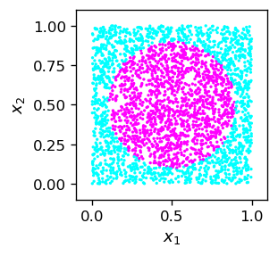
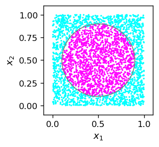
Example with the circle
We illustrate the code on the example of a binary classifier of points inside a circle.
def cir():
    x1=np.random.random()                  # coordinate 1
    x2=np.random.random()                  # coordinate 2
    if((x1-0.5)**2+(x2-0.5)**2 < 0.4*0.4): # inside circle, radius 0.4, center (0.5,0.5)
        return np.array([x1,x2,1])
    else:                                  # outside
        return np.array([x1,x2,0])
For a future use (new convention), we split the sample into separate arrays of features (the two coordinates) and labels (1 if the point is inside the circle, 0 otherwise):
sample_c=np.array([cir() for _ in range(3000)]) # sample
features_c=np.delete(sample_c,2,1)
labels_c=np.delete(np.delete(sample_c,0,1),0,1)
plt.figure(figsize=(2.3,2.3),dpi=120)
plt.xlim(-.1,1.1)
plt.ylim(-.1,1.1)
plt.scatter(sample_c[:,0],sample_c[:,1],c=sample_c[:,2],
            s=1,cmap=mpl.cm.cool,norm=mpl.colors.Normalize(vmin=0, vmax=.9))

plt.xlabel('$x_1$',fontsize=11)
plt.ylabel('$x_2$',fontsize=11)
plt.show()
We choose the following architecture and initial parameters:
arch_c=[2,4,4,1]                  # architecture
weights=func.set_ran_w(arch_c,4)  # scaled random initial weights in [-2,2]
eps=.7                            # initial learning speed
The simulation takes a few minutes,
for k in range(1000):   # rounds
    eps=.995*eps       # decrease learning speed
    if k%100==99: print(k+1,' ',end='')             # print progress
    for p in range(len(features_c)):                # loop over points
        func.back_prop(features_c,labels_c,p,arch_c,weights,eps,
                       f=func.sig,df=func.dsig) # backprop
100 200 300 400 500 600 700 800 900 1000
The reduction of the learning speed in each round gives the final value, which is small, but not too small:
eps
0.004657778005182377
(a too small value would update the weights very little, so further rounds would be useless).
While the learning phase was rather long, the testing is very fast:
test=[]

for k in range(3000):
    po=[np.random.random(),np.random.random()]
    xt=func.feed_forward(arch_c,weights,po,ff=func.sig)
    test.append([po[0],po[1],np.round(xt[len(arch_c)-1][0],0)])

tt=np.array(test)

fig=plt.figure(figsize=(2.3,2.3),dpi=120)

# drawing the circle
ax=fig.add_subplot(1,1,1)
circ=plt.Circle((0.5,0.5), radius=.4, color='gray', fill=False)
ax.add_patch(circ)

plt.xlim(-.1,1.1)
plt.ylim(-.1,1.1)
plt.scatter(tt[:,0],tt[:,1],c=tt[:,2],
            s=1,cmap=mpl.cm.cool,norm=mpl.colors.Normalize(vmin=0, vmax=.9))

plt.xlabel('$x_1$',fontsize=11)
plt.ylabel('$x_2$',fontsize=11)
plt.show()
The trained network looks like this:
fnet=draw.plot_net_w(arch_c,weights,.1)
Note
It is fascinating that we have trained the network to recognize if a point is in a circle, and it has no concept whatsoever of geometry, Euclidean distance, equation of the circle, etc. The network has just learned “empirically” how to proceed, using a training sample!
Note
The result in the plot is pretty good, perhaps except, as always, near the boundary. In view of our discussion of chapter More layers, where we have set the weights of a network with three neuron layers from geometric considerations, the quality of the present result is stunning. We do not see any straight sides of a polygon, but a nicely rounded boundary. As always in these games, improving the result would require a bigger sample and longer training, which is time consuming.
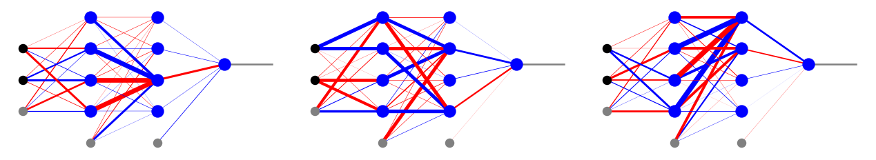
Local minima
We have mentioned before the emergence of local minima in multi-variable optimization as a potential problem. In the figure below we show three different results of the backprop code for our classifier of points in a circle. We note that each of them has a radically different set of optimum weights, whereas the results on the test sample are, at least by eye, equally good for each case. This shows that the backprop optimization ends up, as anticipated, in different local minima. However, each of these local minima works sufficiently well and equally good. This is actually the reason why backprop can be used in practical problems: there are zillions of local minima, but it does not really matter!
General remarks
There are some more important and general observations to be made:
Note
Supervised training of an ANN takes a very long time, but using a trained ANN takes a blink of an eye. The asymmetry originates from the simple fact that the multi-parameter optimization takes very many function calls (here feed-forward) and evaluations of derivatives in many rounds (we have used 1000 for the circle example), but the usage on a point involves just one function call.
A classifier trained with backprop may work inaccurately for the points near the boundary lines. A remedy is to train more for improvement, and/or increase the size of the training sample, in particular near the boundary.
However, a too long learning on the same training sample does not actually make sense, because the accuracy stops improving at some point.
Local minima occur in backprop, but this is by no means an obstacle to the use of the algorithm. This is an important practical feature.
Various improvements of the steepest descent method, or altogether different minimization methods may be used (see exercises). They can largely increase the efficiency of the algorithm.
When going backwards with updating the weights in subsequent layers, one may introduce an increasing factor (see exercises). This helps with performance.
Finally, different activation functions may be used to improve performance (see the following lectures).
Exercises
\(~\)
Prove (analytically) by evaluating the derivative that \( \sigma '(s) = \sigma (s) [1- \sigma (s)]\). Show that the sigmoid is the only function with this property.
Derive backprop formulas for network with one- and two intermediate layers. Note an emerging regularity (recurrence), and prove the general formulas for any number of intermediate layers.
Modify the lecture example of the classifier of points in a circle by replacing the figure with
semicircle;
two disjoint circles;
ring;
any of your favorite shapes.
Repeat 3., experimenting with the number of layers and neurons, but remember that a large number of them increases the computational time and does not necessarily improve the result. Rank each case by the fraction of misclassified points in a test sample. Find an optimum/practical architecture for each of the considered figures.
If the network has a lot of neurons and connections, little signal flows through each synapse, hence the network is resistant to a small random damage. This is what happens in the brain, which is constantly “damaged” (cosmic rays, alcohol, …). Besides, such a network after destruction can be (already with a smaller number of connections) retrained. Take your trained network from problem 3. and remove one of its weak connections (first, find it by inspecting the weights), setting the corresponding weight to 0. Test this damaged network on a test sample and draw conclusions.
Scaling weights in back propagation. A disadvantage of using the sigmoid in the backprop algorithm is a very slow update of weights in layers distant from the output layer (the closer to the beginning of the network, the slower). A remedy here is a re-scaling of the weights, where the learning speed in the layers, counting from the back, is successively increased by a certain factor. We remember that successive derivatives contribute factors of the form \( \sigma '(s) = \sigma (s) [1- \sigma (s)] = y (1-y) \) to the update rate, where \( y \) is in the range \( (0, 1) \). Thus the value of \( y (1-y \) cannot exceed 1/4, and in the subsequent layers (counting from the back) the product \( [y (1-y] ^ n \le 1/4 ^ n\). To prevent this “shrinking”, the learning rate can be multiplied by compensating factors \( 4 ^ n \): \( 4, 16, 64, 256, ... \). Another heuristic argument [RIV91] suggests even faster growing factors of the form \( 6 ^ n \): \( 6, 36, 216, 1296, ... \)
Enter the above two recipes into the code for backprop.
Check if they indeed improve the algorithm performance for deeper networks, for instance for the circle point classifier, etc.
For assessment of performance, carry out the execution time measurement (e.g., using the Python time library packet).
Steepest descent improvement. The method of the steepest descent of finding the minimum of a function of many variables used in the lecture depends on the local gradient. There are much better approaches that give a faster convergence to the (local) minimum. One of them is the recipe of Barzilai-Borwein explained below. Implement this method in the back propagation algorithm. Vectors \(x\) in the \(n\)-dimensional space are updated in subsequent iterations as \( x^{(m + 1)} = x^{(m)} - \gamma_m \nabla F (x^{(m)})\), where \(m\) numbers the iteration, and the speed of learning depends on the behavior at the two (current and previous) points: