Perceptron
Contents
Perceptron
Supervised learning
We have shown in the previous chapters that even the simplest ANNs can carry out useful tasks (emulate logical networks or provide simple memory models). Generally, each ANN has
a certain architecture, i.e. the number of layers, number of neurons in each layer, scheme of connections between the neurons (fully connected or not, feed forward, recurrent, …);
weights (hyperparameters), with specific values, defining the network’s functionality.
The prime practical question is how to set (for a given architecture) the weights such that a requested goal is realized, i.e., a given input yields a desired output. In the tasks discussed earlier, the weights could be constructed a priori, be it for the logical gates or for the memory models. However, for more involved applications we want to have an “easier” way of determining the weights. Actually, for complicated problems a “theoretical” a priori determination of weights is not possible at all. This is the basic reason for inventing learning algorithms, which automatically adjust the weights with the help of the available data.
In this chapter we begin to explore such algorithms with the supervised learning approach, used i.a. for data classification.
Supervised learning
In this strategy, the data must possess labels which a priori determine the correct category for each point. Think for example of pictures of animals (data) and their descriptions (cat, dog,…), which are called the labels. The labeled data are then split into a training sample and a test sample.
The basic steps of supervised learning for a given ANN are following:
Initialize somehow the weights, for instance randomly or to zero.
Read subsequently the data points from the training sample and pass them through your ANN. The obtained answer may differ from the correct one, given by the label, in which case the weights are adjusted according to a specific prescription (to be discussed later on).
Repeat, if needed, the previous step. Typically, the weights are changed less and less as the algorithm proceeds.
Finish the training when a stopping criterion is reached (weights do not change much any more or the maximum number of iterations has been completed).
Test the trained ANN on a test sample.
If satisfied, you have a desired trained ANN performing a specific task (like classification), which can be used on new, unlabeled data. If not, you can split the sample in the training and the test parts in a different way and repeat the procedure from the beginning. Also, you may try to acquire more data (which may be expensive), or change your network’s architecture.
The term “supervised” comes form an interpretation of the procedure where the labels are held by a “teacher”, who thus knows which answers are correct and which are wrong, and who supervises that way the training process. Of course, a computer program “supervises itself”.
Perceptron as a binary classifier
The simplest supervised learning algorithm is the perceptron, invented in 1958 by Frank Rosenblatt. It can be used, i.a., to construct binary classifiers of the data. Binary means that the network is used to assess if a data item has a particular feature, or not - just two possibilities. Multi-label classification is also possible with ANNs (see exercises), but we do not discuss it in these lectures.
Remark
The term perceptron is also used for ANNs (without or with intermediate layers) consisting of the MCP neurons (cf. Fig. Fig. 3 and Fig. 4), on which the perceptron algorithm is executed.
Sample with a known classification rule
To begin, we need some training data, which we will generate as random points in a square. Thus the coordinates of the point, \(x_1\) and \(x_2\), are taken in the range \([0,1]\). We define two categories: one for the points lying above the line \(x_1=x_2\) (call them pink), and the other for the points lying below (blue). During the generation, we check whether \(x_2 > x_1\) or not, and assign a label to each data point equal to, correspondingly, 1 or 0. These labels are “true” answers.
The function generating the above described data point with a label is
def point():     # generates random coordinates x1, x2, and 1 if x2>x1, 0 otherwise
    x1=np.random.random()          # random number from the range [0,1]
    x2=np.random.random()
    if(x2>x1):                     # condition met
        return np.array([x1,x2,1]) # add label 1
    else:                          # not met
        return np.array([x1,x2,0]) # add label 0
We generate a training sample of npo=300 labeled data points:
npo=300 # number of data points in the training sample

print('  x1         x2         label')       # header
samp=np.array([point() for _ in range(npo)]) # training sample, _ is dummy iterator
print(samp[:5, :])                           # first 5 data points
  x1         x2         label
[[0.42111394 0.07020499 0.        ]
 [0.93066523 0.87466665 0.        ]
 [0.90025472 0.34350444 0.        ]
 [0.21285073 0.23776243 1.        ]
 [0.06729928 0.52107458 1.        ]]
Loops in arrays
In Python, one can conveniently define arrays with a loop inside, e.g.
[i**2 for i in range(4)] yields [1,4,9].
In loops, if the index does not explicitly show in the expression, one can use a dummy index _, as for instance in the above code:
[point() for _ in range(npo)]
Ranges in arrays
Not to print unnecessarily the very long table, we have used above for the first time the ranges for array indices. For example, 2:5 means from 2 to 4 (recall the last one is excluded!), :5 - from 0 to 4, 5: - from 5 to the end, and : - all the indices.
Graphically, our data are shown in the figure below. We also plot the line \(x_2=x_1\), which separates the blue and purple points. In this case the division is a priori possible (we know the rule) in an exact manner.
plt.figure(figsize=(2.3,2.3),dpi=120)
plt.xlim(-.1,1.1)                                  # axes limits
plt.ylim(-.1,1.1)
plt.scatter(samp[:,0],samp[:,1],c=samp[:,2],       # label determines the color
            s=5,cmap=mpl.cm.cool)                  # point size and color

plt.plot([-0.1, 1.1], [-0.1, 1.1])                 # separating line

plt.xlabel('$x_1$',fontsize=11)
plt.ylabel('$x_2$',fontsize=11)

plt.show()
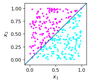
Linearly separable sets
Two sets of points (as here blue and pink) on a plane which are possible to separate with a straight line are called linearly separable. In three dimensions, the sets must be separable with a plane, in general in \(n\) dimensions the sets must must be separable with an \(n-1\) dimensional hyperplane.
Analytically, if the points in the \(n\) dimensional space have coordinates \((x_1,x_2,\dots,x_n)\), one may chose the parameters \((w_0,w_1,\dots,w_n)\) in such a way that one set of points must satisfy the condition
and the other one the opposite condition, with \(>\) replaced with \(\le\).
Now a crucial, albeit obvious observation: the above inequality is precisely the condition implemented in the MCP neuron (with the step activation function) in the convention of Fig. 5! We may thus enforce condition (3) with the neuron function from the neural library.
In our example, we have for the pink points, by construction,
from where, using Eq. (3), we can immediately read out
Thus the neuron function is used on a sample point p as follows:
p=[0.6,0.8]      # sample point with x_2 > x_1
w=[0,-1,1]       # weights as given above

func.neuron(p,w)
1
The neuron fired, so point p is pink.
Observation
A single MCP neuron with properly chosen weights can be used as a binary classifier for \(n\)-dimensional separable data.
Sample with an unknown classification rule
At this point the reader may be a bit misled by the apparent triviality of the results. The confusion may stem from the fact that in the above example we knew from the outset the rule defining the two classes of points (\(x_2>x_1\), or opposite). However, in a general “real life” situation this is usually not the case! Imagine that we encounter the (labeled) data samp2 looking like this:
print(samp2[:5])
[[0.45183395 0.83895895 1.        ]
 [0.9400015  0.18976085 0.        ]
 [0.3524696  0.12013594 0.        ]
 [0.35971149 0.42787117 0.        ]
 [0.47753383 0.98513982 1.        ]]
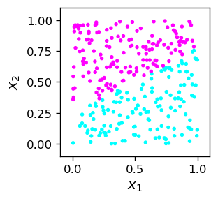
The situation is in some sense inverted now. We have obtained from somewhere the (linearly separable) data, and want to find the rule that defines the two classes. In other words, we need to draw a dividing line, which is equivalent to finding the weights of the MCP neuron of Fig. 5 that would carry out the binary classification.
Perceptron algorithm
We could still try to figure out somehow the proper weights for the present example and find the dividing line, for instance with a ruler and pencil, but this is not the point. We wish to have a systematic algorithmic procedure that will effortlessly work for this one and any similar situation. The answer is the already mentioned perceptron algorithm.
Before presenting the algorithm, let us remark that the MCP neuron with some set of weights \(w_0, w_1, w_2\) always yields some answer for a labeled data point, correct or wrong. For example
w=[-0.5,1,0]           # arbitrary choice of weights

print("label  answer") # header

for i in range(5): # look at first 5 points
    print(int(samp2[i,2]),"    ",func.neuron(samp2[i,:2],w))
            # samp2[i,2] is the label, samp2[i,:2] is [x_1,x_2]
label  answer
1      0
0      1
0      0
0      0
1      0
We can see that some answers are equal to the corresponding labels (correct), and some are different (wrong). The general idea now is to use the wrong answers to adjust cleverly, in small steps, the weights, such that after sufficiently many iterations we get all the answers for the training sample correct!
Perceptron algorithm
We iterate over the points of the training data sample. If for a given point the obtained result \(y_o\) is equal to the true value \(y_t\) (the label), i.e. the answer is correct, we do nothing. However, if it is wrong, we change the weights a bit, such that the chance of getting the wrong answer decreases. The explicit recipe is as follows:
\(w_i \to w_i + \varepsilon (y_t - y_o) x_i\),
where \( \varepsilon \) is a small number (called the learning speed) and \(x_i\) are the coordinates of the input point, with \(i=0,\dots,n\).
Let us follow how it works. Suppose first that \( x_i> 0\). Then if the label \( y_t = 1 \) is greater than the obtained answer \( y_o = 0\), the weight \(w_i\) is increased. Then \( w \cdot x \) also increases and \( y_o = f (w \cdot x) \) is more likely to acquire the correct value of 1 (we remember how the step function \(f\) looks like). If, on the other hand, the label \( y_t = 0 \) is less than the obtained answer \( y_o = 1 \), then the weight \(w_i\) is decreased, \( w \cdot x \) decreases, and \( y_o = f (w \cdot x) \) has a better chance of achieving the correct value of 0.
If \( x_i < 0 \) it is easy to analogously check that the recipe also works properly.
When the answer is correct, \(y_t=y_0\), then \( w_i \to w_i\), so nothing changes. We do not “spoil” the perceptron!
The above formula can be used many times for the same point from the training sample. Next, we loop over all the points of the sample, and the whole procedure can still be repeated in many rounds to obtain stable weights (not changing any more as we continue the procedure, or changing only slightly).
Typically, in such algorithms the learning speed \( \varepsilon \) is being decreased in successive rounds. This is technically very important, because too large updates could spoil the obtained solution.
The Python implementation of the perceptron algorithm for the 2-dimensional data is as follows:
w0=np.random.random()-0.5  # initialize weights randomly in the range [-0.5,0.5]
w1=np.random.random()-0.5
w2=np.random.random()-0.5

eps=.3                     # initial  learning speed

for _ in range(20):        # loop over rounds
    eps=0.9*eps            # in each round decrease the learning speed

    for i in range(npo):   # loop over the points from the data sample

        for _ in range(5): # repeat 5 times for each points

            yo = func.neuron(samp2[i,:2],[w0,w1,w2]) # obtained answer

            w0=w0+eps*(samp2[i,2]-yo)   # weight update (the perceptron formula)
            w1=w1+eps*(samp2[i,2]-yo)*samp2[i,0]
            w2=w2+eps*(samp2[i,2]-yo)*samp2[i,1]

print("Obtained weights:")
print("  w0     w1     w2")        # header
w_o=np.array([w0,w1,w2])           # obtained weights
print(np.round(w_o,3))             # result, rounded to 3 decimal places
Obtained weights:
  w0     w1     w2
[-0.555 -1.109  2.163]
The obtained weights, as we know, define the dividing line. Thus, geometrically, the algorithm produces the dividing line as drawn below, together with the training sample as plotted above.
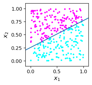
We can see that the algorithm works! All the pink points are above the dividing line, and all the blue ones below. Let us emphasize that the dividing line, given by the equation
does not result from our a priori knowledge, but from the training of the MCP neuron which sets its weights.
Note
One can prove that the perceptron algorithm converges if and only if the data are linearly separable.
We may now reveal our secret! The data of the training sample samp2 were labeled at the time of creation with the rule
which corresponds to the weights \(w_0^c=0.25\), \(w_1^c=-0.52\), \(w_2^c=1\).
w_c=np.array([-0.25,-0.52,1]) # weights used for labeling the training sample
print(w_c)
[-0.25 -0.52 1. ]
Note that these are not at all the same as the weights obtained from the training:
print(np.round(w_o,3))
[-0.555 -1.109 2.163]
The reason is twofold. First, note that the inequality condition (3) is unchanged if we multiply both sides by a positive constant \(c\). We may therefore scale all the weight by \(c\), and the situation (the answers of the MCP neuron, the dividing line) remains exactly the same (we encounter here an equivalence class of weights scaled with a positive factor).
For that reason, when we divide correspondingly the obtained weights by the weights used to label the sample, we get (almost) constant values:
print(np.round(w_o/w_c,3))
[2.22 2.133 2.163]
The reason why the ratio values for \(i=0,1,2\) are not exactly the same is that the sample has a finite number of points (here 300). Thus, there is always some gap between the two classes of points and there is some room for “jiggling” the separating line a bit. With more data points this mismatch effect decreases (see the exercises).
Testing the classifier
Due to the limited size of the training sample and the “jiggling” effect desribed above, the classification result on a test sample is sometimes wrong. This always applies to the points near the dividing line, which is determined with accuracy depending on the multiplicity of the training sample. The code below carries out the check on a test sample. The test sample consists of labeled data generated randomly “on the flight” with the same function point2 used to generate the training data before:
def point2():
    x1=np.random.random()          # random number from the range [0,1]
    x2=np.random.random()
    if(x2>x1*0.52+0.25):           # condition met
        return np.array([x1,x2,1]) # add label 1
    else:                          # not met
        return np.array([x1,x2,0]) # add label 0
The code for testing is as follows:
er= np.empty((0,3))  # initialize an empty 1 x 3 array to store misclassified points

ner=0                 # initial number of misclassified points
nt=10000               # number of test points

for _ in range(nt):   # loop over the test points
    ps=point2()       # a test point
    if(func.neuron(ps[:2],[w0,w1,w2])!=ps[2]): # if wrong answer
        er=np.append(er,[ps],axis=0)           # add the point to er
        ner+=1                                 # count the number of errors

print("number of misclassified points = ",ner," per ",nt," (", np.round(ner/nt*100,1),"% )")
number of misclassified points = 28 per 10000 ( 0.3 % )
As we can see, a small number of test points are misclassified. All these points lie near the separating line.
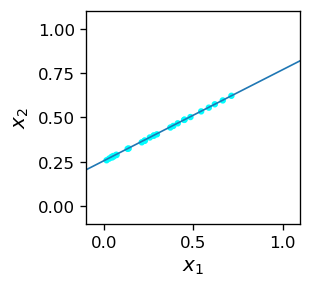
Misclassification
As it became clear, the reason for misclassification comes from the fact that the training sample does not determine the separating line precisely, but with some uncertainty, as there is a gap between the points of the training sample. For a better result, the training points would have to be “denser” in the vicinity of the separating line, or the training sample would have to be larger.
Exercises
\(~\)
Play with the lecture code and see how the percentage of misclassified points decreases with the increasing size of the training sample.
As the perceptron algorithm converges, at some point the weights stop to change. Improve the lecture code by implementing stopping when the weights do not change more than some value when passing to the next round.
Generalize the above classifier to points in 3-dimensional space.