Models of memory
Contents
Models of memory
Heteroassociative memory
Pair associations
We now pass to further illustrations of elementary capabilities of ANNs, describing two very simple models of memory based on linear algebra, supplemented with (nonlinear) filtering. Speaking of memory here, a word of caution is in place. We have rather simplistic tools in mind here, which are far from the actual complex and hitherto not comprehended memory mechanism operating in our brain. The present understanding is that these mechanism involve feed-back, which goes beyond the considered feed-forward networks.
The first considered model concerns the so called heterassociative memory, where some objects (here graphic bitmap symbols) are joined in pairs. In particular, we take the set of five graphical symbols, {A, a, I, i, Y}, and define two pair associations: A \(\leftrightarrow\) a and I \(\leftrightarrow\) i, that is between different (hetero) symbols. Y remains unassociated.
The symbols are defined as 2-dimensional \(12 \times 12\) pixel arrays, for instance
    A = np.array([
       [0, 0, 0, 0, 0, 0, 0, 0, 0, 0, 0, 0],
       [0, 0, 0, 0, 0, 1, 0, 0, 0, 0, 0, 0],
       [0, 0, 0, 0, 0, 1, 0, 0, 0, 0, 0, 0],
       [0, 0, 0, 0, 1, 1, 1, 0, 0, 0, 0, 0],
       [0, 0, 0, 0, 1, 0, 1, 0, 0, 0, 0, 0],
       [0, 0, 0, 1, 0, 0, 0, 1, 0, 0, 0, 0],
       [0, 0, 0, 1, 0, 0, 0, 1, 0, 0, 0, 0],
       [0, 0, 1, 1, 1, 1, 1, 1, 1, 0, 0, 0],
       [0, 0, 1, 0, 0, 0, 0, 0, 1, 0, 0, 0],
       [0, 1, 0, 0, 0, 0, 0, 0, 0, 1, 0, 0],
       [0, 1, 0, 0, 0, 0, 0, 0, 0, 1, 0, 0],
       [0, 0, 0, 0, 0, 0, 0, 0, 0, 0, 0, 0]])
The remaining symbols are defined smilarly.
We use the standard plotting package imported earlier. The whole set of our symbols looks like this, with yellow=1 and violet=0:
sym=[A,a,ii,I,Y] # array of symbols, numbered from 0 to 4
plt.figure(figsize=(16, 6)) # figure with horizontal and vertical size

for i in range(1,6):     # loop over 5 figure panels, i is from 1 to 5
    plt.subplot(1, 5, i) # panels, numbered from 1 to 5
    plt.axis('off')      # no axes
    plt.imshow(sym[i-1]) # plot symbol, numbered from 0 to 4

plt.show()

Warning
In Python, an integer range\((i,j)\) includes \(i\), but does not include \(j\), i.e. equals \([i, i+1, \dots, j-1]\). Also, range\((i)\) includes \(0, 1, \dots, i-1\). This differs from conventions in some other programming languages.
It is more convenient to work not with the above two-dimensional arrays, but with one-dimensional vectors obtained with the so-called flattening procedure, where a matrix is cut along its rows into a vector. For example
t=np.array([[1,2,3],[0,4,0],[3,2,7]]) # a matrix
print(t)
print(t.flatten())                    # matrix flattened into a vector
[[1 2 3]
 [0 4 0]
 [3 2 7]]
[1 2 3 0 4 0 3 2 7]
We thus perform the flattening on our set,
fA=A.flatten()
fa=a.flatten()
fi=ii.flatten()
fI=I.flatten()
fY=Y.flatten()
to obtain, for instance


The advantage of working with vectors is that we can use the scalar product. Note that here the scalar product between two symbols is just equal to the number of common yellow pixels. For instance, for the flattened symbols plotted above we have only two common yellow pixels:
np.dot(fA,fi)
2
It is clear that one can use the scalar product as a measure of similarity between the symbols. For the following method to work, the symbols should not be too similar, as then they could be “confused”.
Memory matrix
The next algebraic concept we need is the outer product. For two vectors \(v\) and \(w\), it is defined as \(v w^T = v \otimes w\) (as opposed to the scalar product, where \(w^T v = w \cdot v\)). Here \(T\) denotes transposition. The result is a matrix with the number of rows equal to the length of \(v\), and the number of columns equal to the length of \(w\).
For example, with
we have
(recall from algebra that we multiply “the rows by the columns”). In numpy
print(np.outer([1,2,3],[2,7])) # outer product of two vectors
[[ 2  7]
 [ 4 14]
 [ 6 21]]
Next, we construct a memory matrix needed for modeling the heteroassociative memory. Suppose first, for simplicity of notation, that we only have two associations: \(a \to A\) and \(b \to B\). Let
Then
and if \(a\) and \(b\) were orthogonal, i.e. \(a \cdot b =0\), then
\( M a = A\)
yielding an exact association. Similarly, we would get \(M b = B\). However, since in a general case the vectors are not exactly orthogonal, an error \(B \, b \cdot a/a \cdot a\) (for the association of \(a\)) is generated. It is usually small if the number of pixels in our symbols is large and the symbols are, loosely speaking, not too similar (do not have too many common pixels. As we will see shortly, the emerging error can be efficiently “filtered out” with an appropriate neuron activation function.
Coming back to our particular case, we thus need four terms in \(M\), as \(a \to A\), \(A\to a\), \(I \to i\), and \(i \to I\):
M=(np.outer(fA,fa)/np.dot(fa,fa)+np.outer(fa,fA)/np.dot(fA,fA)
   +np.outer(fi,fI)/np.dot(fI,fI)+np.outer(fI,fi)/np.dot(fi,fi)); # associated pairs
Now, as a test how it works, for each flattened symbol \(s\) we evaluate \(Ms\). The result is a vector, which we want to bring back to the form of the \(12\times 12\) pixel array. The operation inverse to flattening in Python is reshape. For instance
tt=np.array([1,2,3,5]) # test vector
print(tt.reshape(2,2)) # cutting into 2 rows of length 2
[[1 2]
 [3 5]]
For our vectors we have
Ap=np.dot(M,fA).reshape(12,12)
ap=np.dot(M,fa).reshape(12,12)
Ip=np.dot(M,fI).reshape(12,12)
ip=np.dot(M,fi).reshape(12,12)
Yp=np.dot(M,fY).reshape(12,12) # we also try the unassociated symbol Y

symp=[Ap,ap,Ip,ip,Yp]          # array of associated symbols
For the case of association to A (which should be a), the procedure yields (we use rounding to 2 decimal digits with np.round)
print(np.round(Ap,2)) # pixel map for the association of the symbol A
[[0.   0.   0.   0.   0.   0.   0.   0.   0.   0.   0.   0.  ]
 [0.   0.   0.   0.   0.25 0.85 0.25 0.   0.   0.   0.   0.  ]
 [0.   0.   0.   0.   0.   0.85 0.   0.   0.   0.   0.   0.  ]
 [0.   0.   0.   1.   1.6  1.85 1.89 0.   0.   0.   0.   0.  ]
 [0.   0.   1.   0.   0.6  0.25 1.6  0.   0.   0.   0.   0.  ]
 [0.   0.   1.   0.6  0.   0.54 1.29 0.6  0.   0.   0.   0.  ]
 [0.   0.   1.   0.6  0.   0.25 1.29 0.6  0.   0.   0.   0.  ]
 [0.   0.   0.6  1.6  1.6  1.85 1.89 1.6  0.6  0.   0.   0.  ]
 [0.   0.   0.6  0.   0.   0.25 0.29 0.   0.6  0.   0.   0.  ]
 [0.   0.6  0.   0.   0.   0.25 0.   0.29 0.29 0.6  0.   0.  ]
 [0.   0.6  0.   0.   0.25 0.25 0.25 0.   0.   0.6  0.   0.  ]
 [0.   0.   0.   0.   0.   0.   0.   0.   0.   0.   0.   0.  ]]
We note that the strength of pixels is now not necessarily equal to 0 or 1, as it was in the original symbols. The graphic representation looks as follows:
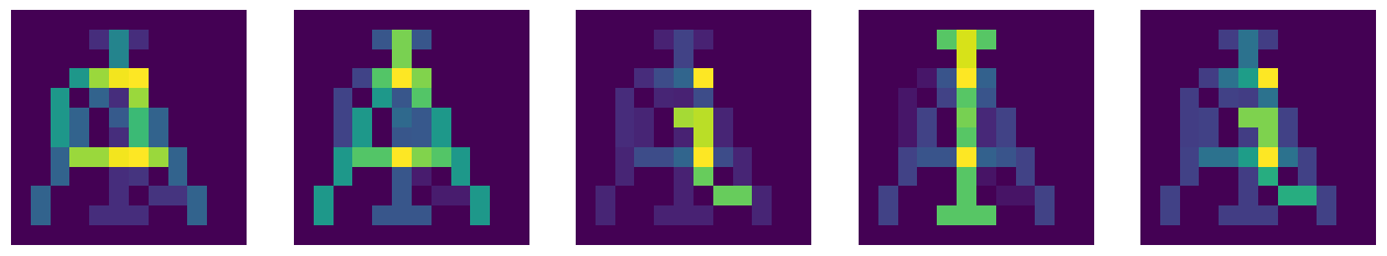
We should be able to see in the above picture the sequence a, A, i, I, and nothing particular in the association of Y. We almost do, but the situation is not perfect due to the nonorthogonality error discussed above.
Applying a filter
The result improves greatly when a filter is applied to the above pixel maps. Looking at the above print out and the plot, we note that we should get rid of the “faint shadows”, and leave only the pixels of sufficient strength, which should then acquire the value 1. In other words, pixels below a bias (threshold) \(b\) should be reset to 0, and those above or equal to \(b\) should be reset to 1. This can be neatly accomplished with our neuron function from Sec. MCP neuron in Python. This function has been placed in the library neural (see Appendix), which we now read in:
We thus define the filter as an MCP neuron with weights \(w_0=-b\) and \(w_1=1\):
def filter(a,b): # a - symbol (2-dim pixel array), b - bias
    n=len(a)     # number of rows (and columns)
    return np.array([[func.neuron([a[i,j]],[-b,1]) for j in range(n)] for i in range(n)])
       # 2-dim array with the filter applied
When operating on Ap with appropriately chosen \(b=0.9\) (the level of the assumed bias is very much relevant). This yields the result
print(filter(Ap,.9))
[[0 0 0 0 0 0 0 0 0 0 0 0]
 [0 0 0 0 0 0 0 0 0 0 0 0]
 [0 0 0 0 0 0 0 0 0 0 0 0]
 [0 0 0 1 1 1 1 0 0 0 0 0]
 [0 0 1 0 0 0 1 0 0 0 0 0]
 [0 0 1 0 0 0 1 0 0 0 0 0]
 [0 0 1 0 0 0 1 0 0 0 0 0]
 [0 0 0 1 1 1 1 1 0 0 0 0]
 [0 0 0 0 0 0 0 0 0 0 0 0]
 [0 0 0 0 0 0 0 0 0 0 0 0]
 [0 0 0 0 0 0 0 0 0 0 0 0]
 [0 0 0 0 0 0 0 0 0 0 0 0]]
where we can notice a “clean” symbol a. We check that it actually works perfectly well for all our associations (such perfection is not always the case):

A representation of the just presented model of the heteroassociative memory in terms of a single-layer network of MCP neurons can be readily given. In the plot below we indicate all the operations, going from left to right. The input symbol is flattened. The input and output layers are fully connected with edges (not shown) connecting the input cells to the neurons in the output layer. The weights of the edges are equal to the matrix elements \(M_{ij}\), indicated with symbol M. The activation function is the same for all neurons and has the form of the step function.
At the bottom, we indicate the elements of the input vector, \(x_i\), of the signal reaching the neuron \(j\), \(s_j=\sum_i x_i M_{ij}\), and the final output \(y_j=f(s_j)\).
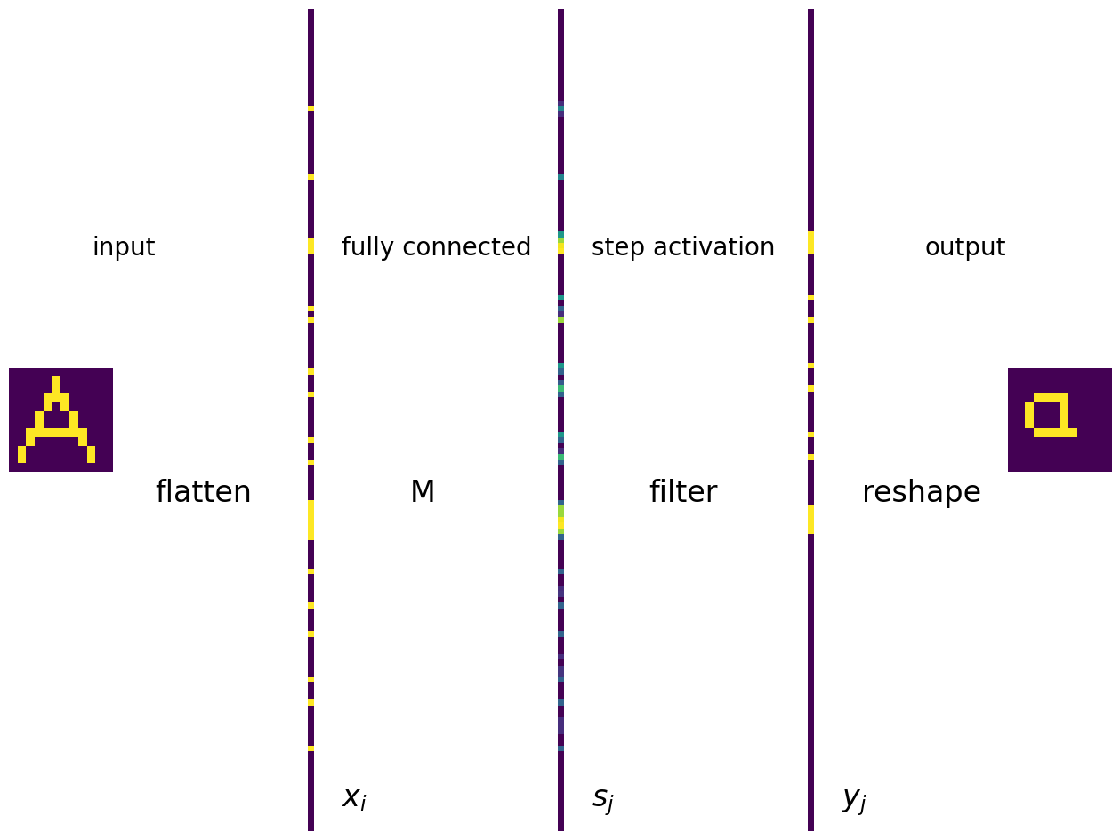
Summary of the model of the heteroassociative memory
Define pairs of associated symbols and construct the memory matrix \(M\).
The input is a symbol in the form of a 2-dim array of pixels with values 0 or 1.
Flatten the symbol into a vector, which forms the layer of inputs \(x_i\).
The weight matrix of the fully connected ANN is \(M\).
The signal entering neuron \(j\) in the output layer is \(s_j=\sum_i x_i M_{ij}\).
The activation (step) function with a properly chosen bias yields \(y_j=f(s_j)\).
Cut the output vector into a matrix of pixels, which constitutes the final output. It should be the symbol associated to the input.
Autoassociative memory
Self-associations
The autoassociative memory model is in close analogy to the case of the heteroassociatine memory, but now the symbol is associated with itself. Why we do such a thing will become clear shortly, when we consider distorted input. We thus define the association matrix as follows:
Ma=(np.outer(fA,fA)/np.dot(fA,fA)+np.outer(fa,fa)/np.dot(fa,fa)
    +np.outer(fi,fi)/np.dot(fi,fi)+np.outer(fI,fI)/np.dot(fI,fI))
After multiplying the flattened symbol with matrix Ma, reshaping, and filtering (all steps as in the heteroassociative case) we properly get back the original symbols (except for Y, which was not associated with anything).

Distorting the image
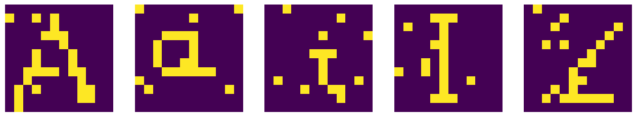
Now imagine that the original image gets partially destroyed, with some pixels randomly altered from 1 to 0 and vice versa. We create a working copy of the original symbols, and next randomly alter some number of pixels (here 8):
sym2=np.copy(sym)                 # copy of symbols

ne=8                              # number of alterations

for s in sym2:                    # loop over symbols
    for _ in range(ne):           # loop over alterations
        i=np.random.randint(0,12) # random row
        j=np.random.randint(0,12) # random column
        s[i,j]=1-s[i,j]           # trick to switch between 1 and 0
After this destruction, the input symbols look like this:
Restoring the symbols
We next apply our model of the autoassociative memory to all the “destroyed” symbols (which are first flattened):
fA2=sym2[0].flatten()
fa2=sym2[1].flatten()
fi2=sym2[2].flatten()
fI2=sym2[3].flatten()
fY2=sym2[4].flatten()
Ap=np.dot(Ma,fA2).reshape(12,12)
ap=np.dot(Ma,fa2).reshape(12,12)
Ip=np.dot(Ma,fI2).reshape(12,12)
ip=np.dot(Ma,fi2).reshape(12,12)
Yp=np.dot(Ma,fY2).reshape(12,12)

symp=[Ap,ap,Ip,ip,Yp]
which yields

After filtering with \(b=0.8\) we obtain back the original symbols:
plt.figure(figsize=(16, 6))

for i in range(1,6):
    plt.subplot(1, 5, i)
    plt.axis('off')
    plt.imshow(filter(symp[i-1],0.8)) # plot filtered symbol

plt.show()

The application of the algorithm can thus decipher a “destroyed” text, or, more generally, provide an error correction mechanism. The method works when there are not too many alterations.
Summary of the model of the autooassociative memory
Construct the memory matrix \(Ma\).
The input is a symbol in the form of a 2-dim array of pixels with values 0 or 1, with a certain number of pixels randomly distorted.
Flatten the symbol into a vector, which forms the layer of inputs \(x_i\).
The weight matrix of the fully connected ANN is \(Ma\).
The signal entering neuron \(j\) in the output layer is \(s_j=\sum_i x_i M_{ij}\).
The activation (step) function with a properly chosen bias yields \(y_j=f(s_j)\).
Cut the output vector into a matrix of pixels, which constitutes the final output. It should bring back the original symbol.
Important
Message: ANNs with one layer of MPC neurons can serve as very simple models of memory!
Note, however, that we constructed the memory matrices algebraically, externally, so to speak. Hence, the network has not really learned the associations from experience. There are ways to do it, but they require more advanced methods (see, e.g., [FS91]), similar to those covered in the following parts of these lectures.
Note
An implementation of the discussed memory models in Mathematica is provided in [Fre93] (https://library.wolfram.com/infocenter/Books/3485) and in the already mentioned lectures by Daniel Kersten.
Exercises
\(~\)
Play with the lecture code and
add more and more symbols;
change the filter level;
increase the number of alterations.
Discuss your findings and the limitations of the models.