Introduction
Contents
Introduction
Purpose of these lectures
The goal of this course is to teach some basics of the omnipresent neural networks with Python [Bar16, Gut16, Mat19]. Both the explanations of key concepts of neural networks and the illustrative programs are kept at a very elementary undergraduate, almost “high-school” level. The codes, made very simple, are described in detail. Moreover, they are written without any use of higher-level libraries for neural networks, which helps in better understanding of the explained algorithms and shows how to program them from scratch.
Who is the book for?
The reader may be a complete novice, only slightly acquainted with Python (or actually any other programming language) and Jupyter.
The material covers such classic topics as the perceptron and its simplest applications, supervised learning with back-propagation for data classification, unsupervised learning and clusterization, the Kohonen self-organizing networks, and the Hopfield networks with feedback. This aims to prepare the necessary ground for the recent and timely advancements (not covered here) in neural networks, such as deep learning, convolutional networks, recurrent networks, generative adversarial networks, reinforcement learning, etc.
On the way of the course, some basic Python programing will be gently sneaked in for the newcomers. Guiding explanations and comments in the codes are provided.
Exercises
At the end of each chapter some exercises are suggested, with the goal to familiarize the reader with the covered topics and the little codes. Most of exercises involve simple modifications/extensions of appropriate pieces of the lecture material.
Literature
There are countless textbooks and lecture notes devoted the matters discussed in this course, hence the author will not attempt to present an even incomplete list of literature. We only cite items which a more interested reader might look at.
With simplicity as guidance, our choice of topics took inspiration from detailed lectures by Daniel Kersten, illustrated in Mathematica, from an on-line book by Raul Rojas (also available in a printed version [FR13]), and the from physicists’ (as myself!) point of view from [MullerRS12].
Biological inspiration
Inspiration for computational mathematical models discussed in this course originates from the biological structure of our neural system [KSJ+12]. The central nervous system (the brain) contains a huge number (\(\sim 10^{11}\)) of neurons, which may be viewed as tiny elementary processor units. They receive a signal via dendrites, and in case it is strong enough, the nucleus decides (a computation done here!) to “fire” an output signal along the axon, where it is subsequently passed via axon terminals to dendrites of other neurons. The axon-dendrite connections (the synaptic connections) may be weak or strong, modifying the passed stimulus. Moreover, the strength of the synaptic connections may change in time (Hebbian rule tells us that the connections get stronger if they are being used repeatedly). In this sense, the neuron is “programmable”.
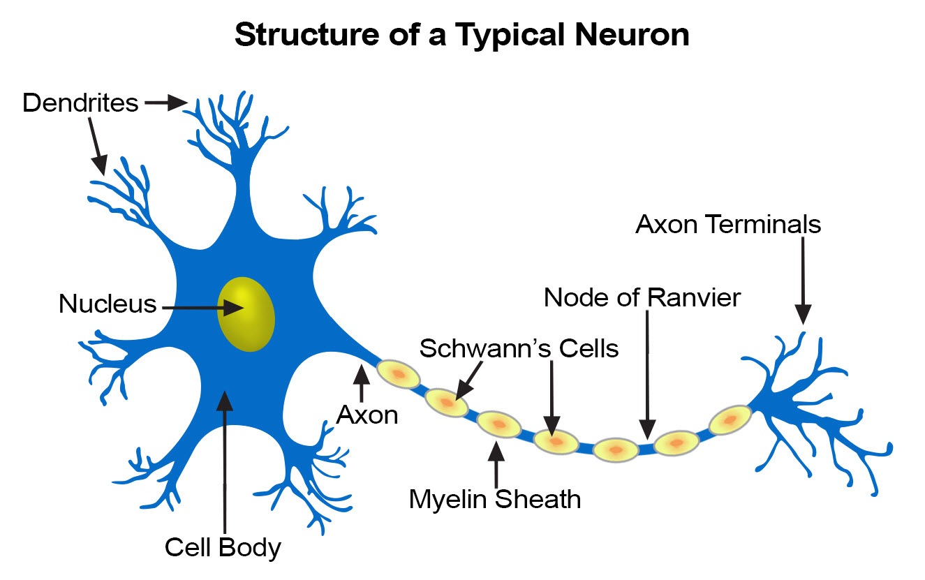
Fig. 1 Biological neuron (from https://training.seer.cancer.gov/anatomy/nervous/tissue.html).
We may ask ourselves if the number of neurons in the brain should really be termed so “huge” as usually claimed. Let us compare it to the computing devices with memory chips. The number of \(10^{11}\) neurons roughly corresponds to the number of transistors in a 10GB memory chip, which does not impress us so much, as these days we may buy such a device for 2$ or so.
Moreover, the speed of traveling of the nerve impulses, which is due to electrochemical processes, is not impressive, either. Fastest signals, such as those related to muscle positioning, travel at speeds up to 120m/s (the myelin sheaths are essential to achieve them). The touch signals reach about 80m/s, whereas pain is transmitted only at comparatively very slow speeds of 0.6m/s. This is the reason why when you drop a hammer on your toe, you sense it immediately, but the pain reaches your brain with a delay of ~1s, as it has to pass the distance of ~1.5m. On the other hand, in electronic devices the signal travels along the wires at speeds of the order of the speed of light, \(\sim 300000{\rm km/s}=3\times 10^{8}{\rm m/s}\)!
For humans, the average reaction time is 0.25s to a visual stimulus, 0.17s to an audio stimulus, and 0.15s to a touch. Thus setting the threshold time for a false start in sprints at 0.1s is safely below a possible reaction of a runner. These are extremely slow reactions compared to electronic responses.
Based on the energy consumption of the brain, one can estimate that on the average a cortical neuron fires about once per 6 seconds. Likewise, it is unlikely that an average cortical neuron fires more than once per second. Multiplying the firing rate by the number of all the cortical neurons, \(\sim 1.6 \times 10^{10}\), yields about \(3 \times 10^{9}\) firings/s in the cortex, or 3GHz. This is the rate of a typical processor chip! Hence if the firing is identified with an elementary calculation, the thus defined power of the brain is comparable to that of a standard computer processor.
The above facts might indicate that, from a point of view of naive comparisons with silicon-based chips, the human brain is nothing so special. So what is it that gives us our unique abilities: amazing visual and audio pattern recognition, thinking, consciousness, intuition, imagination? The answer is linked to an amazing architecture of the brain, where each neuron (processor unit) is connected via synapses to, on the average, 10000 (!) other neurons. This feature makes it radically different and immensely more complicated than the architecture consisting of a control unit, processor, and memory in our computers (the von Neumann machine architecture). There, the number of connections is of the order of the number of bits of the memory. In contrast, there are about \(10^{15}\) synaptic connections in the human brain. As mentioned, the connections may be “programmed” to get stronger or weaker. If, for the sake of a simple estimate, we approximated the connection strength by just two states of a synapse, 0 or 1, the total number of combinatorial configurations of such a system would be \(2^{10^{15}}\) - a humongous number. Most of such configuration, of course, never realize in practice, nevertheless the number of possible configuration states of the brain, or the “programs” it can run, is truly immense.
In recent years, with developing powerful imaging techniques, it became possible to map the connections in the brain with unprecedented resolution, where single nerve bundles are visible. The efforts are part of the Human Connectome Project, with the ultimate goal to map one-to-one the human brain architecture. For the much simpler fruit fly, the drosophila connectome project is very well advanced.
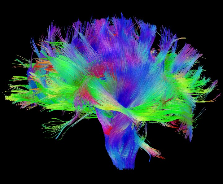
Fig. 2 White matter fiber architecture of the brain (from the Human Connectome Project humanconnectomeproject.org)
Important
The “immense connectivity” feature, with zillions of neurons serving as parallel elementary processors, makes the brain a completely different computational device from the Von Neumann machine (i.e. our everyday computers).
Feed-forward networks
The neurophysiological research of the brain provides important guidelines for mathematical models used in artificial neural networks (ANNs). Conversely, the advances in algorithmics of ANNs frequently bring us closer to understanding of how our “brain computer” may actually work!
The simplest ANNs are the so called feed forward networks, exemplified in Fig. 3. They consist of an input layer (black dots), which just represents digitized data, and layers of neurons (colored blobs). The number of neurons in each layer may be different. The complexity of the network and the tasks it may accomplish increase, naturally, with the number of layers and the number of neurons.
In the remaining part of this section we give, in a rather dense format, a bunch of important definitions:
Networks with one layer of neurons are called single-layer networks. The last layer (light blue blobs) is called the output layer. In multi-layer (more than one neuron layer) networks the neuron layers preceding the output layer (purple blobs) are called intermediate layers. If the number of layers is large (e.g. as many as 64, 128, …), we deal with the recent “ground-breaking” deep networks.
Neurons in various layers do not have to function the same way, in particular the output neurons may act differently from the others.
The signal from the input travels along the links (edges, synaptic connections), indicated with arrows, to the neurons in subsequent layers. In feed-forward networks, as the one in Fig. 3, it can only move forward (from left to right in the figure): from the input to the first neuron layer, from the first to the second, and so on until the output is reached. No going backward to preceding layers, or parallel propagation among the neurons of the same layer, are allowed. This would be a recurrent feature that we touch upon in section Lateral inhibition.
As we describe in detail in the following chapters, the traveling signal is appropriately processed by the neurons, hence the device carries out a computation: input is being transformed into output.
In the sample network of Fig. 3 each neuron from a preceding layer is connected to each neuron in the following layer. Such ANNs are called fully connected.
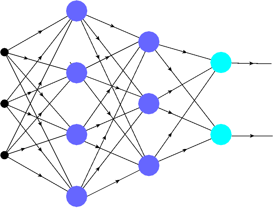
Fig. 3 A sample feed-foward fully connected artificial neural network. The colored blobs represent the neurons, and the edges indicate the synaptic connections. The signal propagates starting from the input (black dots), via the neurons in subsequent intermediate (hidden) layers (purple blobs), to the output layer (light blue blobs). The strength of the connections is controled by weights (hyperparameters) assigned to the edges.
As we will discuss in greater detail shortly, each edge (synaptic connection) in the network has a certain “strength” described with a number called weight (the weights are also termed hyperparameters). Even very small fully connected networks, such as the one of Fig. 3, have very many connections (here 30), hence contain a lot of hyperparameters. Thus, while sometimes looking innocuously, ANNs are in fact very complex multi-parametric systems. Moreover, a crucial feature here is an inherent nonlinearity of the neuron responses, as we discuss in chapter MCP Neuron.
Why Python
The choice of Python for the little codes of this course needs almost no explanation. Let us only quote Tim Peters:
Beautiful is better than ugly.
Explicit is better than implicit.
Simple is better than complex.
Complex is better than complicated.
Readability counts.
According to SlashData, there are now over 10 million developers in the world using Python, just second after JavaScript (~14 million). In particular, it proves very practical in applications to ANNs.
Imported packages
Throughout this course we use some standard Python library packages for the numerics, plotting, etc. As stressed, we do not use any libraries specifically dedicated to neural networks. Each lecture’s notebook starts with the inclusion of some of these libraries:
import numpy as np              # numerical
import statistics as st         # statistics
import matplotlib.pyplot as plt # plotting
import matplotlib as mpl        # plotting
import matplotlib.cm as cm      # contour plots

from mpl_toolkits.mplot3d.axes3d import Axes3D   # 3D plots
from IPython.display import display, Image, HTML # display imported graphics
neural package
Functions created during this course which are of repeated use, are placed in the private library package neural, described in appendix neural package.
For compatibility with Google Colab, the lib_nn package is imported in the following way:
import os.path

isdir = os.path.isdir('lib_nn') # check whether 'lib_nn' exists

if not isdir:
   !git clone https://github.com/bronwojtek/lib_nn.git # cloning the library from github

import sys
sys.path.append('./lib_nn')

from neural import *            # importing my library package
Note
For brevity of presentation, some redundant (e.g. imports of libraries) or inessential pieces of the code are present only in the downloadable source Jupyter notebooks, and are not included/repeated in the book. This makes the text more concise and readable.