MCP Neuron
Contents
MCP Neuron
Definition
We need a basic building block of ANNs: the artificial neuron. The first mathematical model dates back to Warren McCulloch and Walter Pitts (MCP)[MP43], who proposed it in 1942, hence at the very beginning of the electronic computer age during World War II. The MCP neuron depicted in Fig. 4 is a basic ingredient of all ANNs discussed in this course. It is built on very simple general rules, inspired neatly by the biological neuron:
The signal enters the nucleus via dendrites from other neurons.
The synaptic connection for each dendrite may have a different (and adjustable) strength (weight).
In the nucleus, the signal from all the dendrites is combined (summed up) into \(s\).
If the combined signal is stronger than a given threshold, then the neuron fires along the axon, in the opposite case it remains still.
In the simplest realization, the strength of the fired signal has two possible levels: on or off, i.e. 1 or 0. No intermediate values are needed.
Axon terminal connects to dendrites of other neurons.
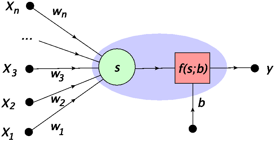
Fig. 4 MCP neuron: \(x_i\) is the input, \(w_i\) are the weights, \(s\) is the signal, \(b\) is the bias, and \(f(s;b)\) represents an activation function, yielding the output \(y=f(s;b)\). The blue oval encircles the whole neuron, as used e.g. in Fig. 3.
Translating this into a mathematical prescription, one assigns to the input cells the numbers \(x_1, x_2 \dots, x_n\) (input data point). The strength of the synaptic connections is controlled with the weights \(w_i\). Then the combined signal is defined as the weighted sum
The signal becomes an argument of the activation function, which, in the simplest case, takes the form of the step function
When the combined signal \(s\) is larger than the bias (threshold) \(b\), the nucleus fires. i.e. the signal passed along the axon is 1. in the opposite case, the generated signal value is 0 (no firing). This is precisely what we need to mimic the biological prototype.
There is a convenient notational convention that is frequently used. Instead of splitting the bias from the input data, we may treat all uniformly. The condition for firing may be trivially transformed as
where \(x_0=1\) and \(w_0=-b\). In other words, we may treat the bias as a weight on the edge connected to an additional cell with the input always fixed to 1. This notation is shown in Fig. 5. Now, the activation function is simply
with the summation index in \(s\) starting from \(0\):
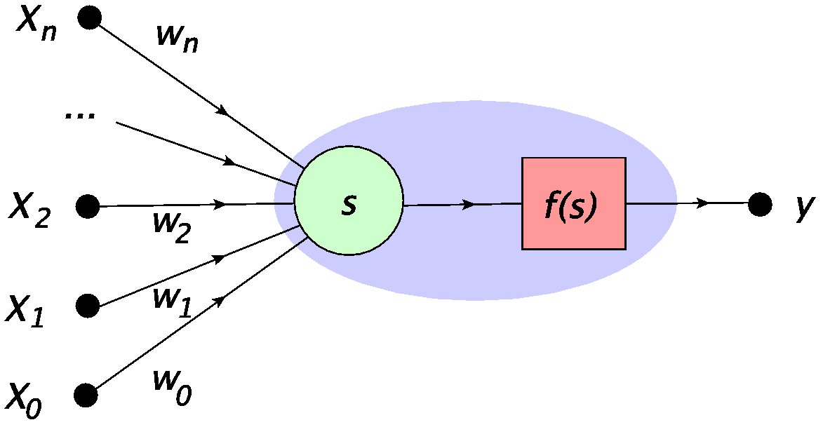
Fig. 5 Alternative, more uniform representation of the MCP neuron, with \(x_0=1\) and \(w_0=-b\).
Hyperparameters
The weights \(w_0=-b,w_1,\dots,w_n\) are generally referred to as hyperparameters. They determine the functionality of the MCP neuron and may be changed during the learning (training) process (see the following). However, they are kept fixed when using the trained neuron on a particular input data sample.
Important
An essential property of neurons in ANNs is nonlinearity of the activation function. Without this feature, the MCP neuron would simply represent a scalar product, and the feed-forward networks would just involve trivial matrix multiplications.
MCP neuron in Python
We now implement the mathematical model of the neuron of Sec. MCP Neuron in Python. First, we obviously need arrays (vectors), which are represented as
x = [1,3,7]
w = [1,1,2.5]
and (important) are indexed starting from 0, e.g.
x[0]
1
(note that typing a variable at the end of a notebook cell prints out its content). The numpy library functions carry the prefix np, which is the alias given at import. Note that these functions act distributively over arrays, e.g.
np.sin(x)
array([0.84147098, 0.14112001, 0.6569866 ])
which is a very convenient feature when programming. We also have the scalar product \(x \cdot w = \sum_i x_i w_i\) handy, which we use to build the combined signal \(s\) entering the MCP neuron:
np.dot(x,w)
21.5
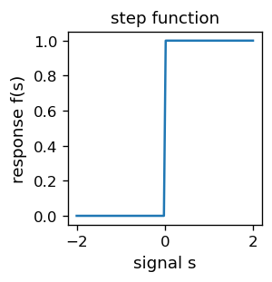
Next, we need to construct the neuron activation function, which presently is just the step function (1):
def step(s):       # step function
     if s > 0:     # condition satisfied
        return 1
     else:         # otherwise
        return 0
where in the top comments we have indicated that the function is also defined in the neural library package, cf. Appendix. For the visualizers, the plot of the step function is following:
plt.figure(figsize=(2.3,2.3),dpi=120) # set the size and resolution of the figure

s = np.linspace(-2, 2, 100)   # array of 100+1 equally spaced points in [-2, 2]
fs = [step(z) for z in s]     # corresponding array of function values

plt.xlabel('signal s',fontsize=11)      # axes labels
plt.ylabel('response f(s)',fontsize=11)
plt.title('step function',fontsize=11)  # plot title

plt.plot(s, fs)
plt.show()
Since \(x_0=1\) always, we do not want to explicitly carry this over in the arguments of functions that will follow. We will be frequently inserting \(x_0=1\) into the input, for instance:
x=[5,7]
np.insert(x,0,1) # insert 1 in x at position 0
array([1, 5, 7])
Now we are ready to construct the MCP neuron:
def neuron(x,w,f=step): # (in the neural library)
    """
    MCP neuron

    x: array of inputs  [x1, x2,...,xn]
    w: array of weights [w0, w1, w2,...,wn]
    f: activation function, with step as default

    return: signal=weighted sum w0 + x1 w1 + x2 w2 +...+ xn wn = x.w
    """
    return f(np.dot(np.insert(x,0,1),w)) # insert x0=1 into x, output f(x.w)
We diligently put the comments in triple quotes to be able to get a useful help when needed:
help(neuron)
Help on function neuron in module __main__:

neuron(x, w, f=<function step at 0x7fe444256550>)
    MCP neuron

    x: array of inputs  [x1, x2,...,xn]
    w: array of weights [w0, w1, w2,...,wn]
    f: activation function, with step as default

    return: signal=weighted sum w0 + x1 w1 + x2 w2 +...+ xn wn = x.w
Note that function f is an argument of neuron. It is by default set to step, thus does not have to be present in the argument list. A sample usage with \(x_1=3\), \(w_0=-b=-2\), \(w_1=1\) is
neuron([3],[-2,1])
1
As we can see, the neuron fired in this case, because \(s=1*(-2)+3*1>0\).
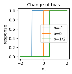
Next, we show how the neuron operates on an input sample \(x_1\) taken in the range \([-2,2]\). We also change the bias parameter, to illustrate its role. It is clear that the bias works as the threshold: if the signal \(x_1 w_1\) is above \(b=-x_0\), then the neuron fires.
plt.figure(figsize=(2.3,2.3),dpi=120)

s = np.linspace(-2, 2, 200)
fs1 = [neuron([x1],[1,1]) for x1 in s]      # more function on one plot
fs0 = [neuron([x1],[0,1]) for x1 in s]
fsm12 = [neuron([x1],[-1/2,1]) for x1 in s]

plt.xlabel('$x_1$',fontsize=11)
plt.ylabel('response',fontsize=11)

plt.title("Change of bias",fontsize=11)

plt.plot(s, fs1, label='b=-1')
plt.plot(s, fs0, label='b=0')
plt.plot(s, fsm12, label='b=1/2')
plt.legend()     # legend
plt.show()
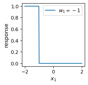
When the sign of the weight \(w_1\) is negative, we get a reverse behavior, where the neuron fires when \(x_1 |w_1| < w_0\):
Note
From now on, for the brevity of the presentation, we hide some cells of the code with repeated structure. The reader may find the complete code in the corresponding Jupyter notebooks.
Admittedly, in the last example, one departs from the biological pattern, as negative weights are not possible to realize in a biological neuron. However, this freedom enriches the mathematical model, which clearly can be built without biological constraints.
Boolean functions
Having constructed the MCP neuron in Python, the question is: What is the simplest (but still non-trivial) application we can use it for? We show here that one can easily construct boolean functions, or logical networks, with the help of networks of MCP neurons. Boolean functions, by definition, have arguments and values in the set \(\{ 0,1 \}\), or {True, False}.
To warm up, let us start with some guesswork, where we take the neuron with the weights \(w=[w_0,w_1,w_2]=[-1,0.6,0.6]\) (why not). We shall here denote \(x_1=p\), \(x_2=q\), in accordance with the traditional notation for logical variables, where \(p,q \in \{0,1\}\).
print("p q n(p,q)") # print the header
print()             # print space

for p in [0,1]:       # loop over p
    for q in [0,1]:   # loop over q
        print(p,q,"",neuron([p,q],[-1,.6,.6])) # print all cases
p q n(p,q)

0 0  0
0 1  0
1 0  0
1 1  1
We immediately recognize in the above output the logical table for the conjunction, \(n(p,q)=p \land q\), or the logical AND operation. It is clear how the neuron works. The condition for the firing \(n(p,q)=1\) is \(-1+p*0.6+q*0.6 \ge 0\), and it is satisfied if and only if \(p=q=1\), which is the definition of the logical conjunction. Of course, we could have used here 0.7 instead of 0.6, or in general \(w_1\) and \(w_2\) such that \(w_1<1, w_2<1, w_1+w_2 \ge 1\). In the electronics terminology, we can call the present neuron the AND gate.
We can thus define the short-hand
def neurAND(p,q): return neuron([p,q],[-1,.6,.6])
Quite similarly, we may define other boolean functions (or logical gates) of two logical variables. In particular, the NAND gate (the negation of conjunction) and the OR gate (alternative) are realized with the following MCP neurons:
def neurNAND(p,q): return neuron([p,q],[1,-0.6,-0.6])
def neurOR(p,q):   return neuron([p,q],[-1,1.2,1.2])
They correspond to the logical tables
print("p q  NAND OR") # print the header
print()

for p in [0,1]:
    for q in [0,1]:
        print(p,q," ",neurNAND(p,q)," ",neurOR(p,q))
p q  NAND OR

0 0   1   0
0 1   1   1
1 0   1   1
1 1   0   1
Problem with XOR
The XOR gate, or the exclusive alternative, is defined with the following logical table:
This is one of the possible boolean functions of two arguments (in total, we have 16 different functions of this kind, why?). We could now try very hard to adjust the weights in our neuron to make it behave as the XOR gate, but we are doomed to fail. Here is the reason:
From the first row of the above table, it follows that for the input 0, 0 (first row) the neuron should not fire. Hence
\(w_0 + 0* w_1 + 0*w_2 < 0\), or \(-w_0>0\).
For the cases of rows 2 and 3 the neuron must fire, therefore
\(w_0+w_2 \ge 0\) and \(w_0+w_1 \ge 0\).
Adding side-by-side the three obtained inequalities we get \(w_0+w_1+w_2 > 0\). However, the fourth row yields \(w_0+w_1+w_2<0\) (no firing), so we encounter a contradiction. Therefore no choice of \(w_0, w_1, w_2\) exists to do the job!
Important
A single MCP neuron cannot represent the XOR gate.
XOR from composition of AND, NAND and OR
One can solve the XOR problem by composing three MCP neurons, for instance
def neurXOR(p,q): return neurAND(neurNAND(p,q),neurOR(p,q))
print("p q XOR")
print()

for p in [0,1]:
    for q in [0,1]:
        print(p,q,"",neurXOR(p,q))
p q XOR

0 0  0
0 1  1
1 0  1
1 1  0
The above construction corresponds to the simple network of Fig. 6.
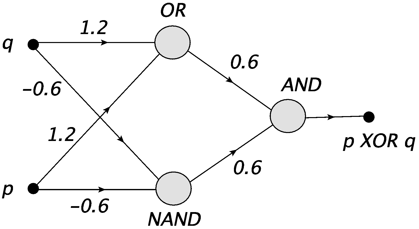
Fig. 6 The XOR gate composed of the NAND, OR, and AND MCP neurons.
Note that we are dealing here, for the first time, with a network having an intermediate layer, consisting of the NAND and OR neurons. This layer is indispensable to construct the XOR gate.
XOR composed from NAND
Within the theory of logical networks, one proves that any network (or any boolean function) can be composed of only NAND gates, or only the NOR gates. One says that the NAND (or NOR) gates are complete. In particular, the XOR gate can be constructed as
[ p NAND ( p NAND q ) ] NAND [ q NAND ( p NAND q ) ],
which we can write in Python as
def nXOR(i,j): return neurNAND(neurNAND(i,neurNAND(i,j)),neurNAND(j,neurNAND(i,j)))
print("p q XOR")
print()

for i in [0,1]:
    for j in [0,1]:
        print(i,j,"",nXOR(i,j))
p q XOR

0 0  0
0 1  1
1 0  1
1 1  0
Note
One proves that logical networks are complete in the Church-Turing sense, i.e., (when sufficiently large) may carry over any possible calculation. This feature directly carries over to ANNs. Historically, that was the basic finding of the seminal MCP paper [MP43].
Conclusion
ANNs (sufficiently large) can perform any calculation!
Exercises
\(~\)
Construct (all in Python)
a gate realizing conjunction of multiple boolean variables;
gates NOT, NOR;
gates OR, AND, NOT by composing NAND gates;
as networks of MCP neurons.